Understanding Support Vector Machine
The last blog you need to understand SVM
- What is SVM?
In Machine Learning, out of the many available supervised classification algorithms, Support Vector Machine (SVM) is one of the easiest algorithm and yet sometimes it becomes difficult to grasp due to its little nuances. In this blog, I try to lay down my notes on unboxing the SVM blackbox and make it easy to understand in detail. This blog focusses on entirety of SVM, from its introduction to classification and kernel tricks.
The idea of SVM is simple: The algorithm creates a line or a hyperplane that separates data into different classes. Let’s understand how SVM creates the hyperplane and what are its other jargon.
What is SVM?
Support Vector Machine (SVM) is a supervised ML algorithm that can be used for classification and regression as well. However, it is mostly used in classification problems.
In SVM classificatio, each data point is plotted in an n-dimensional space (n = Nos. of features). and classified by finding the best hyperplane that differentiates the classes well.
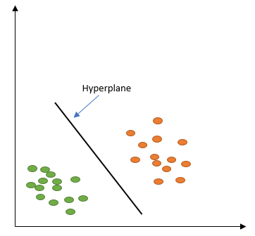
In the above image, data points are plotted in a 2-dimensional space and solid black line is the hyperplane that is able to divide the dataset in two classes viz. orange and green color. The hyperplane becomes the decision boundary where if datapoints are above the hyperplane( black line) they belong to orange class and if datapoints are below the hyperplane they belong to green class.
Hyperplanes are n-1 -dimensional planes where n is total number of features of the dataset. From the above image, data is 2 dimensional and hyperplane divding the space is a 1 dimensional plane.
Taking it further: in the above example there is a hyperplane drew that differentiates the dataset in two classes very well. But on keenly thinking, there are other possible hyperplanes too which could be selected that divides the dataset. Something like in the image below:

Apart from the black coloured hyperplane line, there are other infinite hyperplanes available(to name a few: red, blue, yellow) which could differentiate the dataset too. But which is the best hyperplane among all and what is the criteria to call a hyperplane best? This question is answered with the help of Support Vectors.
What are Support Vectors?
Support Vectors are the vectors passing through the closest data points to the hyperplanes and are parallel to the hyperplane. The distance between the support vectors and hyperplane is called as margin. The thumb rule to identify the right hyperplane among infinitly available hyperplanes is: “Select the hyper-plane which segregates the two classes better such that the margin is maximum between the support vector and hyperplane”.
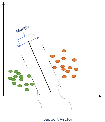
In above image, the middle solid black colored line is the hyperplane that divides the dataset into classes whereas two parallel dashed lines are its support vectors and they pass through the closest datapoints to the hyperplane.
The margin is maximum ever possible due to these chosen support vectors and hence the hyperplane derived from it is the best hyperplane to classify the datapoints into classes.
Few points on Support Vectors:
1. The data/vector points closest to the hyperplane are known as **support vector** data points because only these two points are contributing to the result of SVM, other points are not.
2. If a data point is not an support vector, removing it has no effect on the model.
3. Deleting the support vector will change the position of the hyperplane.
Intuition for Large Margins
In SVM, the classification is not done based on the hyperplane decision boundary but even support vectors are also considered in classification. The region between two support vectors which includes hyperplane becomes the decision region. In fig. 3, if datapoints are above the decision region towards right they will be classified into orange class and if datapoints are below the decision region towards left they will be classified into green class.
Maximizing the margin seems good because data points near the decision region represent very uncertain classification decisions. For example, after training SVM we got a certain hyperplane with its support vectors such that the margin is very-very small. In this case SVM does not have confidence on its prediction of datapoints which are very close to the decsision region: there is almost a $50\%$ chance of the classifier deciding either way. Whereas a SVM classifier with a large margin makes no low certainty classification decisions. A large margin gives classifier safety margin where a slight error in measurement or a slight document variation will not cause a misclassification.
Mathematics for SVM
Lets go through the mathematics of SVM and understand SVM manages to select the hyperplane with maximum margin possible.
Generally, the equation of a line is given by: $y=ax+b$. We should define the hyperplane equation with this equation but however, we will define the equation of hyperplane in this form: $W^TX = 0$. Lets see how these two forms are related.
In hyperplane equation the names of the variables are in bold which means that that they are vectors and $W^TX$ represent the inner product(i.e. dot product) of two vectors.
Note that is same as . We can write: $W = \begin{bmatrix}-b\cr-a\cr1\end{bmatrix}$ and $X = \begin{bmatrix}1 \cr x \cr y \end{bmatrix}$. Then:
The two equations are just different ways of expressing the same thing. It is interesting to note that is which determines the intersection of the line with the vertical axis.
We use hyperplane equation $W^TX$ instead as $y=ax+b$ for two reasons:
- it is easier to work in more than two dimensions with this notation,
- the vector $W$ will always be normal to hyperplane ($W$ will always be normal because it is used to define the hyerplane, so by definition it will be normal. More Info Here)
Compute distance from a point to the hyperplane
In Fig. 4, there is a hyperplane that divides two sets of data. Here, there is no Y-intercept i.e. $w_0 = 0$.
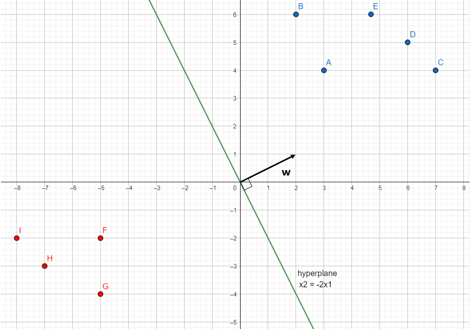
As can be seen from Fig. 4, the equation of hyperplane is: which is equivalent to with $W = \begin{bmatrix}2\cr1\end{bmatrix}$ and $X = \begin{bmatrix}x_1\cr x_2\end{bmatrix}$. Note that vector $W$ is shown in the figure.
We would like to compute the distance between point $A(3,4)$ and the hyperplane. This is the distance between $A$ and its projection onto the hyperplane.
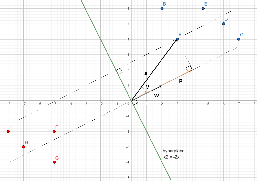
We can view point $A$ as a vector from the origin to $A$. If we project this vector $A$ onto $W$ we get vector $P$. The distance between point $A(3,4)$ and hyperplane is same as $||p||$. We will be finding $||p||$.
Let $u$ denote the direction of vector $W$ which is given by $u = \frac{W}{||w||}$.
. So, $u$ becomes $u = \begin{bmatrix}\frac{2}{\sqrt{5}}, \frac{1}{\sqrt{5}}\end{bmatrix}$.
To compute $||p||$, we need to find value of vector $P$. From, the figure we can conclude that $P$ is the orthogonal projection of $A$ onto $W$.
The dot product between $A$ and $W$ is: $A.W = ||a|| \times ||w|| \cos\theta \Longrightarrow \cos\theta = \frac{A.W}{||a|| \times ||w||}$
If we apply, Pythagoras theorem in the above figure we will also get: $\cos\theta = \frac{||p||}{||a||}$.
Equating above two equations:
We already know that:
Substituting $u$ in tha above equation
Vector $P$ is in same direction as vector $W$. Hence, we can define $u$ in terms of vector $p$ as well:
So,
Compute the margin of hyperplane
Now that we have distance $||p||$ between $A$ and hyperplane, the margin is defined by:
Finding the optimal-best hyperplane
In above section, we first considered a hyperplane that divided the dataset into two classes. We took closest point to this hyperplane i.e.point $A$, as one of the support vector will pass through it and calculated its ($||p||$) distance from the hyperplane. With $margin = 2 \times ||p|$ we would get two support vectors and hyperplane as shown below:
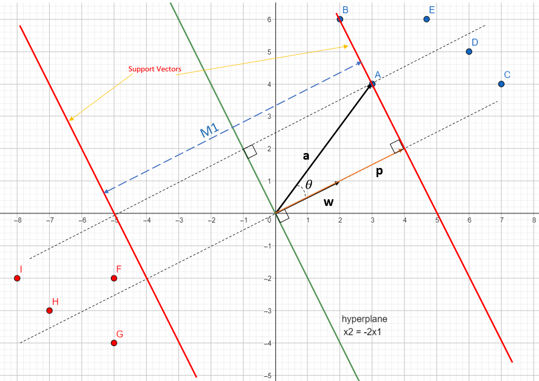
As we have seen earlier, the best hyperplane is the one with the maximum margin. In Fig. 4, the margin $M_1$ between two red support vectors is not the biggest margin possible. The biggest margin is margin $M_2$ with a different hyperplane which is the optimal one is shown in Fig. 5:
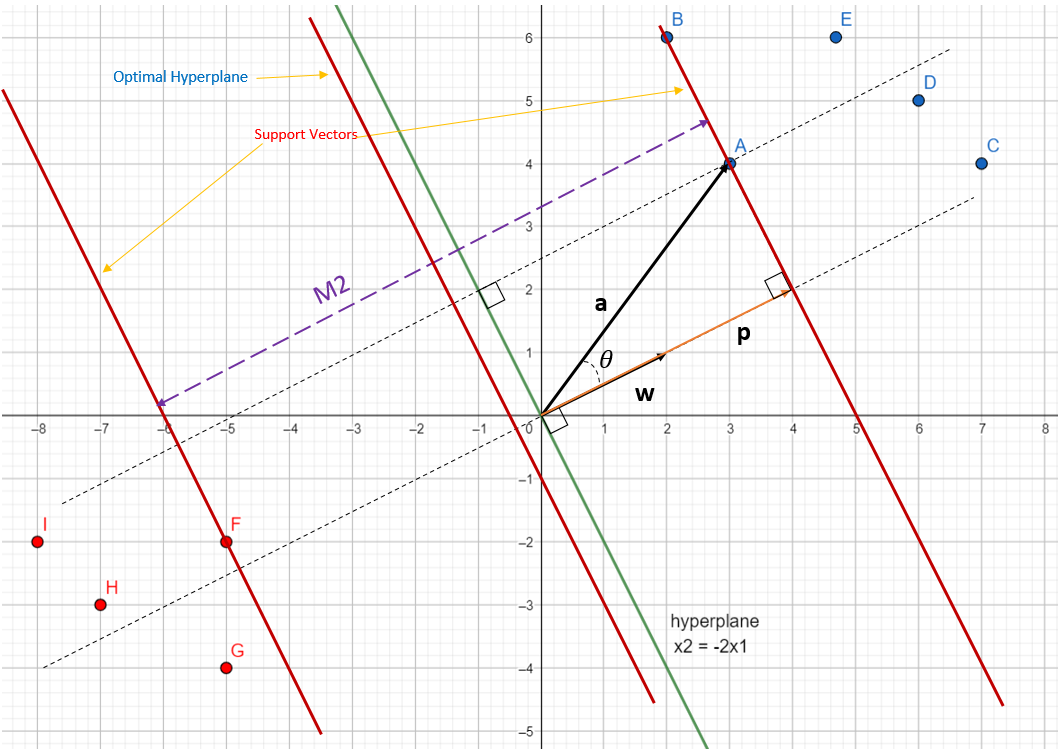
Optimal hyperplane is slightly left of the initial hyperplane that we considered. It is found by simply tracing a line crossing $M_2$ in its middle. We can say that margins and hyperplanes are closely related and one can be found from another:
If we have hyperplane we can compute its margin with respect to some data point. If we have margin delimited by two support vectors, we can find the hyperplane passing right in the middle of the margin.
Finding the biggest margin is same as finding the best optimal hyperplane
Finding biggest margin
The biggest margin can be found in following steps:
1. Take a dataset.
2. Select two hyperplanes(referring to support vectors here) which separate the data with no points between them
3. Maximize the distance (margin)
Step 1: Defining the dataset
Usually, the dataset consists of $n$ datapoints of $X_i$. Each $X_i$ is associated with a value $y_i$ inidicating the element belongs to the class($+1$) or not($-1$).
.
Moreover, each vector $X_i$ consists of lot of dimensions. Lets say that $X_i$ is a $p$-dimensional vector. So dataset $D$ is the set of $n$ couples of element $(X_i, y_i)$. The more formal definition of dataset is:
Step 2: Selecting two hyperplanes with no data points between them
We need to find two hyperplanes with the help of datapoints such that there are no datapoints between these two hyperplanes. These two hyperplanes are actually the support vectors and with the help of these we will derive the optimal hyperplane.
In the previous examples above, the datapoints were linearly separable and the hyperplane could be easily identified with the eye itself by visualisation. With dataset being non-linearly separable (like shown below) it becomes difficult to identify the hyperplane that divides the dataset. Moreover, whenever data is of $p$-dimension it becomes ever more difficult.
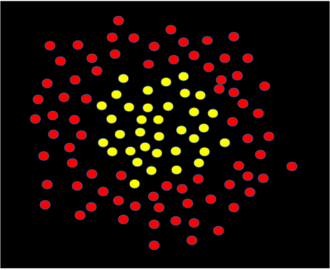
So let’s assume dataset $D$ is linearly separable and we would want to find two hyperplanes with no points between them without visualisation.
We saw earlier, equation of hyperplane can be written as: $W^{T}X = 0$. We will change this equation notation to:
Not that in earlier hyperplane equation, vector $W$ contains $b$ but in new notation, $b$ has been taken out. $W^{T}X$ and $W.X$ both represent dot product. Both equations represent hyperplane and are same equations just that they are in different notations. The new equation has been used going forward.
Given a hyperplane $H_o$ separating the dataset and satisfying:
We can select two other hyperplanes $H_1$ and $H_2$ which also separates the data and have the following equations:
and
so that $H_o$ is equidistant from $H_1$ and $H_2$.
Here, the variable $\delta$ is not necessary and so to simply we can set it to $1$. So,
With the help of above hyperplane equations, we will select the hyperplanes which satisfies the following constraints:
For each vector $X_i$ either:
Understanding the constraints
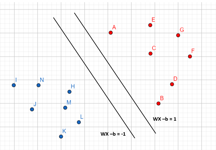
In the following figures, all the red data points belong to class 1 whereas all blue data points belong to class -1.
Consider we have two hyperplanes with equations $W.X_i + b = 1$ and $W.X_i + b = - 1$ and all the datapoints follows the constraints as described above.
Let’s look at Fig. 6 below and consider the point A. It is red so it belong to class 1 and we need to verify it does not violate constraint $W.X_i + b \geq 1$. When $X_i = A$, we see that the point is on the hyperplane and so $W.X_i + b = 1$ and the constraint is respected. Same goes for $B$. When $X_i = C$, we see the point is above the hyperplane so $W.X_i + b \ge 1$ and the constraint is respected. The same applied for $D,\space E,\space F$ and $G$.
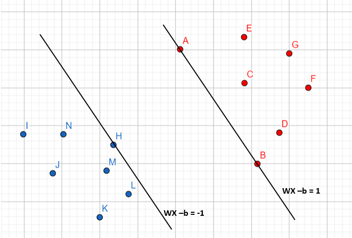
With an analogous reasoning we can see second constraint is respected for class -1.
There is another set of hyperplanes that respects the constraints:
Let’s see when constraints are not being respected. Below image shows sequences of instances where constraints are not followed:
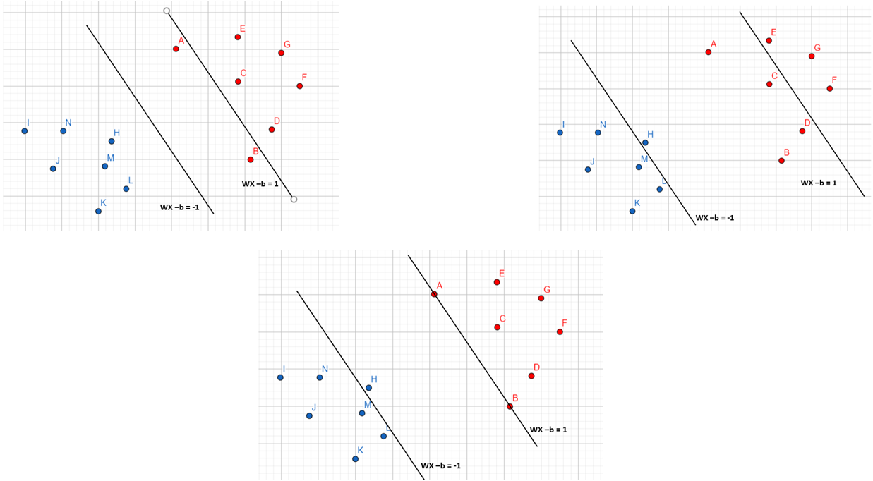
Whenever, the constraints are not being followed we cannot select those two hyperplanes. In every failed instances above, there are datapoints between the two sets of hyperplanes which we don’t want.
Let’s combine two constraints into one equation for simplicity.
Starting with equation (2)
Multiply both sides with $y_i$ (which is $-1$ for this equation)
In equation (1), multiply both sides with $y_i$ and as $y_i =1$, sign of inequation doesn’t change
Nw we can combine equations (3) and (4) and have one equation for both the constraints
We now have a unique constraint in equation (5) instead of two equations (1), (2).
Step 3: Maximize distance between two hyperplanes
Let’s find the distance between two hyperplanes first.
Let:
- $H_o$ be the hyperplane having equation $W.X + b = -1$
- $H_1$ be the hyperplane having equation $W.X + b = 1$
- $x_o$ be a point on hyperplane $H_0$
We will call $m$ the perpendicular distance from $x_o$ to the hyperplane $H_1$. By definition, $m$ is the $margin$ and hence $m$ is the distance between hyperplane $H_o$ and $H_1$.
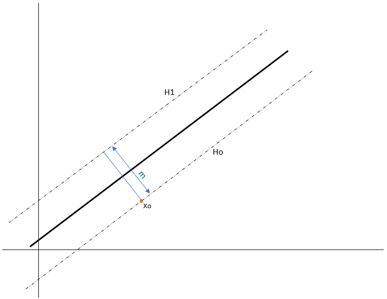
To find $m$, we would find a vector such that:
- has magnitude of $m$
- it is perpendicular to hyperplane $H_1$
Fortunately, we already know a vector perpendicular to $H_1$, i.e. vector $W$ (because $H_1 = W.X + b = 1$)
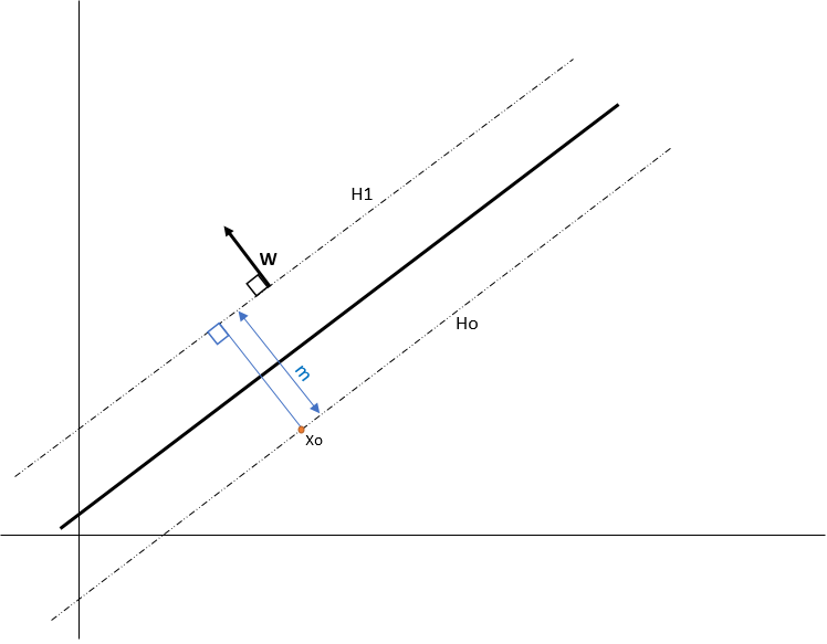
Lets define $u = \frac{W}{||W||}$ as the unit vector of $W$. As its a unit vector, $||u|| = 1$ and it has the same direction as $W$, so it is also perpendicular to $H_1$.
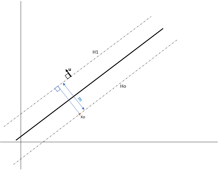
If we multiply $u$ by scalar $m$ we get the vector $k = m u $ and
- $||k|| = m$
- $k$ is perpendicular to $H_1$ (because it has the same direction as $u$)
From these properties we can see that $k$ is the vector we are looking for:
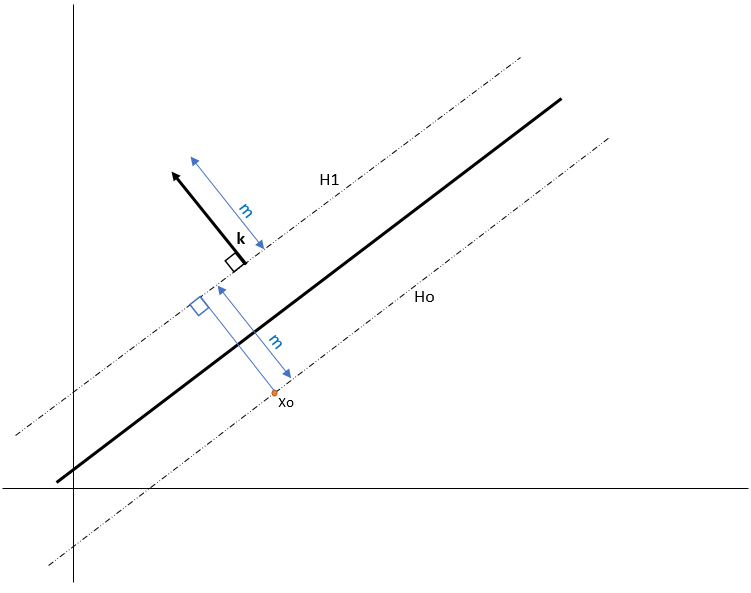
If we start from the point $X_o$ and add $k$ we find that the point $Z_o = X_o + k$ is in the hyperplane $H_1$ as shown in below figure:
The fact that $Z_o$ lies on $H_1$ means that:
Replacing $k$ with equation (6):
The dot product of a vector with itself is the square of its norm so:
As $X_o$ is on $H_o$ then $W.X_o + b = -1$
So, we got the equation to compute the margin: . Our goal is to maximize the margin $m$. This could be achieved by minimizing $W$.
Once we minimize the $||W||$, we maximize the margin $m$ and hence we would find our optimal hyperplane lying in middle fof $H_o$ and $H_1$. To make the problem easier when taking the gradients, we will try to minimize the following form:
Linear Inseparability
All the examples we have seen until so far were linear separable i.e., the data points could be classified with a straight line (or hyperplane). In real world, dataset is not easy to classify with just a hyperplane and are often linear inseparable. Look at one of the examples of linear inseparable data below:
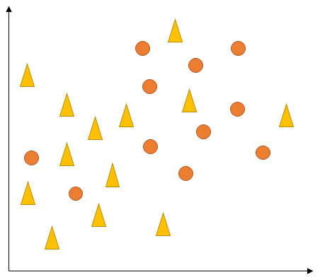
From the Fig. 13, it is evident that there is no linear decision boundary exists that can perfectly segregate the data i.e. the data is linearly inseparable. We have similar situations in higher-dimensional representations as well. These could be solved easily with either soft-margin formulation or kernel trick.
Soft Margin Formulation
In real life, data is messy and cannot be segregated perfectly with a hyperplane. Due to this, the constraint of maximizing the margin of the line that separates the classes must be relaxed. For example, consider the following diagram:
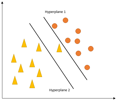
In above image, hyperplane 1 perfectly segregates all the training datapoints and respects the constraints of the support vectors i.e. no data point between the support vectors hyperplanes. Due to this constraint, we have a small margin. But, is it really a good idea of having a decision boundary that perfectly separates datapoints with such less margin? The answer is NO. If we consider hyperplane 2 in above image, it gives a bigger margin but have a misclassification of yellow traingle. So which hyperplane is better? Hyperplane 2 is a better decision boundary as it has a wider margin and thus is able to generalize well on the unseen data. Hyperplane 2 though misclassifying one of the datapoints but this error is acceptable in the broad sense of generalizing the data well.
The concept of margins where support vectors doesn't allow any data points to lie between them is called hard-margin. Hard-margins in SVM are prone to be influenced even by the single outlier (like in image above) which makes the classifier overly sensitive to the noise in data and overfits the data.
Soft-margins in SVM allows the misclassification to a certain extent(hyperplane 2 in above image) while training and deciding decision boundary hyperplane and generalizes well on the data.
How Soft Margin works mathematically?
As explained earlier, for SVM to work, the objective function is equation no. (7). In the new setting of soft margin, objective function from equation no. (7) can be modified as below:
This differs from the original objective function in the second term. Here, $C$ is a hyperparameter that decides the trade-off between maximizing the margin and minimizing the misclassifications. When, $C$ is small, classification errors are given less importance and focus is more on maximizing the margin which will lead to SVM overfitting on the dataset. Whereas when $C$ is large, the focus is more on avoiding misclassifications at the expense of keeping the margin small which means that there will be misclassifications allowed while training such that the margin got is not small but big enough to generalize the data very well.
However, not all misclassification mistakes are equal. Since, decision hyperplane boundary is made based on computation of distances among data points, we also need to consider the distances while considering the misclassification mistakes. Data points that are far away on the wrong side of the decision hyperplane boundary should incur more penalty as compared to the ones that are closer. Let’s see how this is incorporated with the help of following image:
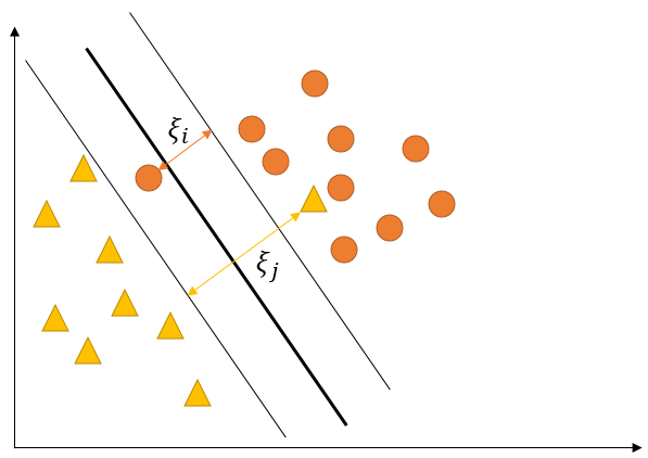
The idea is: for every data point $X_i$, there is a slack variable introduced $\xi_{i}$. The $\xi_{i}$ represents distance of $X_i$ from the corresponding class’ margin if $X_i$ is on the wrong side of the margin, otherwise zero. Thus the points that are far away from the margin on the wrong side would get more penalty.
With this idea, each data point $X_i$ needs to satisfy the following constraint:
The objective function to minimize with soft-margin setting becomes:
Refereces