Quantization: A Deep Dive into Model Compression

Introduction

Imagine you want to run Llama 2 70B on your machine. There’s just one problem: in its native FP32 precision, the model weights alone take up roughly 280GB of RAM memory and additional memory of around 20GB for context which grows with sequence length. That’s more than most high-end GPUs can handle, let alone a laptop.

Now what if you could shrink the model down to 35GB or even 17GB without losing much of its quality?

That’s what quanitzation does. It is the process of reducing the numerical precision of a model’s weights and activations (for e.g. converting 32-bit floating point numbers to 8-bit integers) so that model gets smaller and its need less memory and compute to run.

To understand how quantization works, we need to start with the foundation: how are numbers actually stored in neural networks? The storage format determines both the precision we get and the memory consumed.#

Number Representation & Data Types

Before we can shrink a model, we need to understand what we are shrinking. AI models internally perform mathematical operations on weights and activations, and how those parameters are stored determines both the precision & accuracy of the results and the memory model consumes.

Weights & activations are stored in floating point format, which has three components:

• Sign bit: Indicates whether the number is positive or negative.
• Exponent: Determines the range of the number (how large or small it can be).
• Mantissa (or significant): Represents the precision of the number (how many decimal places it can have).

More bits means more room for the exponent and mantissa, which allows for a wider range of values and greater precision. For example, FP32 (32-bit floating point) has 1 sign bit, 8 bits for the exponent, and 23 bits for the mantissa, while FP16 (16-bit floating point) has 1 sign bit, 5 bits for the exponent, and 10 bits for the mantissa.

Precision refers to the number of significant figures or decimal places a number can represent. In floating point numbers, precision is determined by the mantissa—more bits in the mantissa mean finer granularity and better accuracy for decimal values.

Bits Spectrum

Here’s how the common data types compare:

Data Type	Total Bits	Sign Bits	Exponent Bits	Mantissa Bits	Range of Values	Memory Usage
FP32	32	1	8	23	~-3.40e38 to ~3.4e38	4 bytes
FP16	16	1	5	10	-65504 to 65504	2 bytes
BF16	16	1	8	7	~−3.38e38 to ~3.38e38	2 bytes
INT8	8	0	0	8	-128 to 127	1 byte
INT4	4	0	0	4	-8 to 7	0.5 byte
INT2	2	0	0	2	-2 to 1	0.25 byte
INT1	1	0	0	1	-1 to 0	0.125 byte

A few things to notice:

• FP16 halves the memory usage of FP32 but sacrifices both range and precision. This can cause overflow issues during training when gradients get very large.
• BF16 is an interesting compromise: it keeps the same exponent (and thereof range) as FP32 but has less precision than FP16. This makes it more effective for training because gradient magnitudes are preserved even if the values are slightly less precise.
• INT8 and lower integer formats (INT4, INT2, INT1) are integer formats where there is no exponent, no mantissa, just whole numbers within a fixed rrange. They’re much cheaper to compute with but can’t represent the same nuance as floating point formats.

As you can see, as we reduce the number of bits, we also reduce the range and precision of the values we can represent. This is the trade-off that quantization makes: by using fewer bits, we can save memory and computational resources, but we may lose some accuracy in the process.

How Memory Is Calculated

Each parameter is a model is stored as a number in a given data type, and each data type uses a fixed number of bits. So, the memory usage of a model can be calculated using the formula:

\(\text{Memory Usage} = \frac{\text{Number of Parameters} \times \text{Bits per Parameter}}{8} \text{ bytes}\) Where:

• Number of Parameters is the total number of weights and biases in the model.
• Bits per Parameter is the number of bits used to represent each parameter (e.g., 32 for FP32, 16 for FP16, 8 for INT8, etc.).
• We divide by 8 to convert bits to bytes.

Let’s take a 7 billion parameter model as an example:

Data Type	Bits per Parameter	Calculation	Memory Usage (GB)
FP32	32	(7e9 * 32) / 8	28 GB
FP16	16	(7e9 * 16) / 8	14 GB
BF16	16	(7e9 * 16) / 8	14 GB
INT8	8	(7e9 * 8) / 8	7 GB
INT4	4	(7e9 * 4) / 8	3.5 GB
INT2	2	(7e9 * 2) / 8	1.75 GB
INT1	1	(7e9 * 1) / 8	0.875 GB

As you can see, by reducing the precision of the data type, we can significantly reduce the memory usage of the model, especially for large models with billions of parameters, where the memory requirements can quickly become unmanageable.

Seeing it in Code-Action

import torch

model = torch.randn(1000,1000) # A simple tensor

print(f"FP32: {model.element_size() * model.nelement() / 1e6:.2f} MB")
print(f"FP16: {model.half().element_size() * model.nelement() / 1e6:.2f} MB")
print(f"INT8: {model.char().element_size() * model.nelement() / 1e6:.2f} MB")

# Outputs
FP32: 4.00 MB
FP16: 2.00 MB
INT8: 1.00 MB

In this example, we create a random tensor of shape (1000, 1000) which has 1 million elements. We then calculate the memory usage for FP32, FP16, and INT8 formats. As you can see, the memory usage decreases as we reduce the precision of the data type. Same tensor, same shape but 4x less memory just by changing the data type. Now if we scale this to a model with billions of parameters, the memory savings become significant, allowing us to run larger models on hardware with limited resources.

Now we understood the different data types and how they impact memory usage. One might think: “Okay, just use INT8 and save memory!”. But it’s not that simple. One can’t just convert FP32 values directly to INT8 - their ranges are completely different. PF32 can represent values from -3.4e38 to 3.4e38m while INT8 only goes from -128 to 127. We need a systemic way to map enormous FP32 range down to the tiny INT8 range without losing too much information. That systemic way is what quantization schemes are all about.

Quantization Schemes

In practice, we do not need to map the entire FP32 range [-3.4e38, 3.4e38] to the smaller range of INT8 [-128, 127]. Instead, we need to find a way to map the range of our data (the model’s parameters and activations) to the smaller range of the target data type.

Symmetric & Asymmetric Quantization are two common schemes for doing this mapping and are forms of linear mapping.

Symmetric Quantization

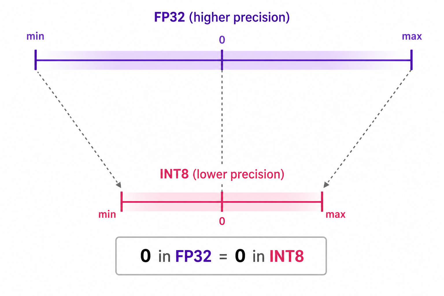
In symmetric quantization, the range of the original values is mapped to a symmetric range around zero in the quantized space. This means that the quantized value for zero in the original data type space is exactly zero in the quantized space.

An example of symmetric quantization is absolute maximum (absmax) quantization, where given a list of values, the highest absolute value ($\alpha$) is taken as the range to perform the linear mapping, as shown in the diagram below:

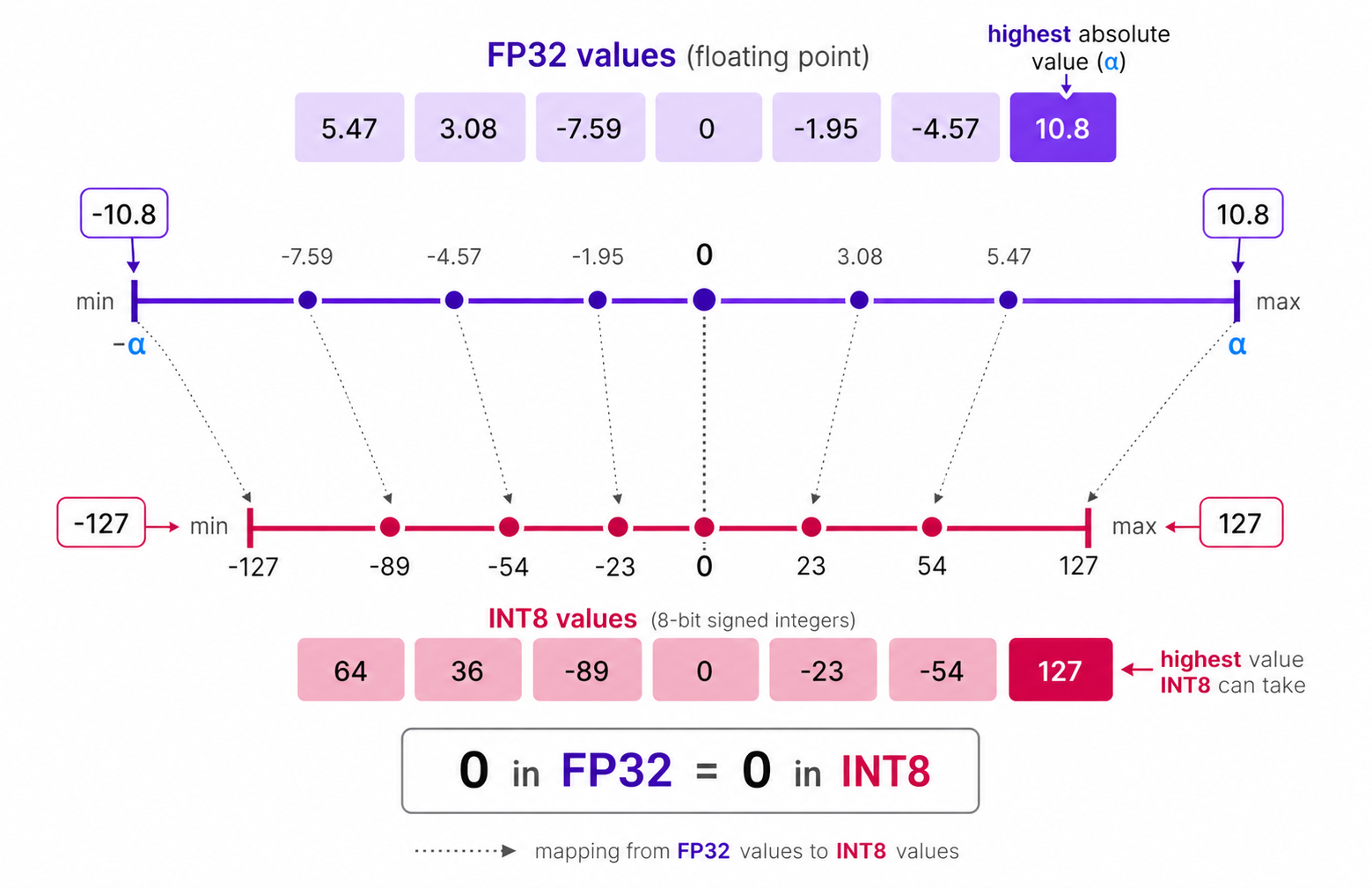
Among the given list of values, $10.8$ is the highest absolute value, so $\alpha$ is set to $10.8$ and while quantizing the FP-32 to INT-8, $10.8$ will be mapped to $127$ and $-10.8$ will be mapped to $-127$ while maintianing symmetry around $0$.

Symmetric Quantization Algorithm

Since it is a linear mapping centered around zero, the process of quantization is straightforward.

We first calculate the scale factor ($s$) which determines how much we need to scale down the original values to fit into the range of the target data type. The formula for calculating the scale factor in symmetric quantization is:

\(S = \frac{2^{b-1} - 1}{\alpha}\) Where:

• $S$ is the scale factor.
• $b$ is the number of bits in the target data type (e.g., 8 for INT8).
• $\alpha$ is the maximum absolute value in the original data (e.g., the weights or activations).

Then, we can quantize the original value ($x$) to the quantized value ($q$) using the formula:

\[X_{quantized} = \text{round}({S}\times{X})\]

Filling in the values would give us:

\[S = \frac{2^{8-1} - 1}{10.8} = \frac{127}{10.8} \approx 11.76\] \[X_{quantized} = \text{round}(11.76 \times X)\]

Asymmetric Quantization

In asymmetric quantization, the mapping is not centered around zero. Instead, it maps the minimum $\beta$ and maximum $\alpha$ values of the original data to the minimum and maximum values of the quantized data type, respectively.

The method we are going to explore is called zero-point quantization.

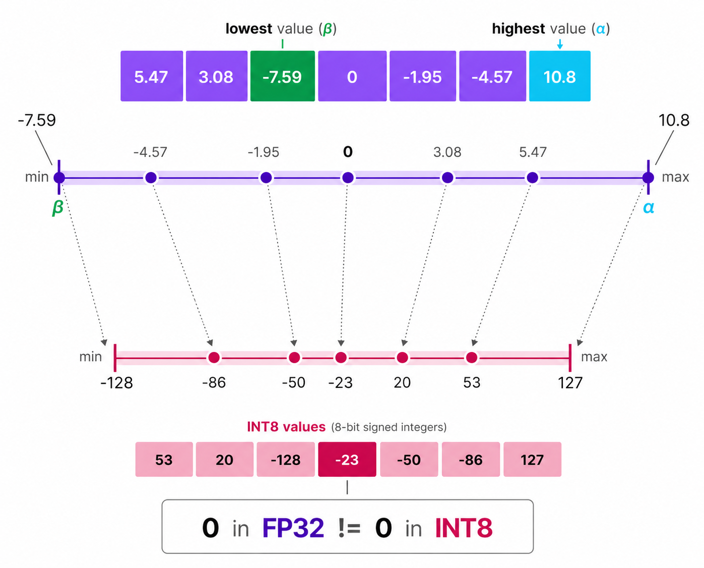
Notice how the $0$ has shifted positions? That’s why its called asymmetric quantization. The min/max values have different distances to 0 in the range [-7.59, 10.8]

Asymmetric Quantization Algorithm

Due to its shifted position, we have to calculate the zero-point for the INT8 range to perform the linear mapping. We also calculate the scale factor using the difference between INT8’s max and min values.

The formula for calculating the scale factor in asymmetric quantization is:

\[\begin{aligned}& S = \frac{128 - -127}{\alpha - \beta} = \frac{255}{\alpha - \beta}\\ \text{where:}\\ & S\text{ is the scale factor.}\\ & \alpha\text{ is the maximum value in the original data.}\\ & \beta\text{ is the minimum value in the original data.}\\ \end{aligned}\]

Then, we calculate the zero-point ($Z$) using the formula:

\[Z = \text{round}(-S \times \beta) - 2^{b-1}\]

Finally, we can quantize the original value ($X$) to the quantized value ($X_{quantized}$) using the formula:

\[X_{quantized} = \text{round}(S \times X) + Z\]

Filling in the values would give us:

\[\begin{aligned}& S = \frac{255}{10.8 - (-7.59)} = \frac{255}{17.39} \approx 13.86\\ & Z = \text{round}(-13.86 \times -7.59) - 128 = \text{round}(105.17) - 128 = 105 - 128 = -23\\ & X_{quantized} = \text{round}(13.86 \times X) - 23 \end{aligned}\]

The dequantization process (converting back to the original data type) is done using the formula:

\[\begin{aligned} & X_{dequantized} = \frac{X_{quantized} - Z}{S} \\ \text{where: }\\ & X_{dequantized} \text{ is the dequantized value.}\\ & X_{quantized} \text{ is the quantized value.} \end{aligned}\]

Range Mapping & Clipping

In previous examples of symmetric and asymmetric quantization, we explored how the range of values in a given vector are mapped to a lower-bit representation. This approach allows full range of vector values to be mapped but it introduces a significant downside: outliers.

Suppose there is a vector with the following values:

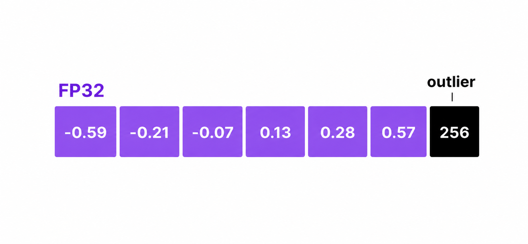
Notice that one value is significantly larger than the others and effectively acting as an outlier. When we perform quantization, the presence of this outlier will cause the scale factor to be much smaller, which means that the other values will be mapped to a very narrow range in the quantized space. This can lead to a significant loss of information for those values, as they will all be mapped to the same or similar quantized value.

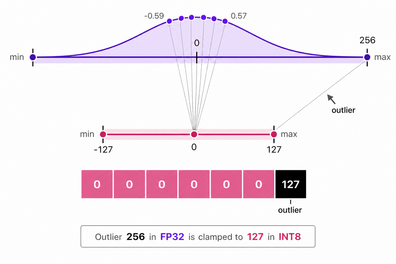
In the above image, the outlier value $(256)$ causes the scale factor be be very small, which leads to all other smaller values getting mapped to the same lower-bit representation (e.g., 0 in INT8), resulting in a loss of information of those values.

To fix this, we can choose to clip certain values. Clipping involves setting a different range of the original values such that all outliers get the same value. In the example below, if we were to manually set the range to [-5, 5] all values outside that will be either mapped to $-127$ or to $127$ regardless of their value.

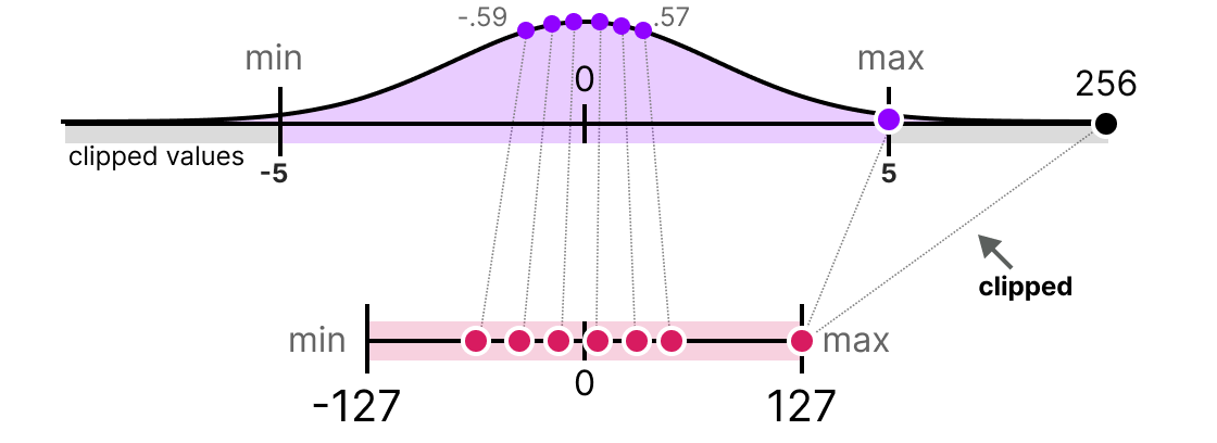
In the above image, by clipping the original data values to a range of [-5, 5], we can mitigate the impact of the outlier (256) and allow the other values to be mapped to a wider range in the quantized space, thus preserving more information about those values.

Calibration

The process of determining the appropriate clipping range is called calibration. Calibration can be done using different methods, such as:

• Percentile Calibration: This method uses percentiles of the data to determine the clipping range. For example, we can choose to clip values above the 99th percentile and below the 1st percentile. This method is more robust to outliers, as it focuses on the distribution of the majority of the data rather than being influenced by extreme values.
• KL Divergence Calibration: This method uses the Kullback-Leibler divergence to measure the difference between the original data distribution and the quantized data distribution. The clipping range is determined by minimizing the KL divergence, which helps to preserve the overall distribution of the data in the quantized space.
• MSE Calibration: This method uses the mean squared error to measure the difference between the original data and the quantized data. The clipping range is determined by minimizing the MSE, which helps to preserve the accuracy of the quantized values compared to the original values.

Performing calibration step is not same for all types of parameters. Weights are fixed after training, so theur range can be computed directly from the weight values - no input data needed. Activations, however, change with every input, so calibration requires running a representative dataset through the model to observe the actual range of values each layer produces at runtime.

Per-Tensor vs Per-Channel Quantization

So far, every example we’ve seen has used a single scale factor for an entire set of values. But when quantizing a real model, you have a choice of granularity - how boradly or narrowly you apply that scale. This choice has a significant impact on accuracy.

Per-Tensor Quantization

Per-tensor quantization uses a single factor and zero-point for the entire weight tensor of a layer. Every single weight value in that layer gets mapped using the same scale.

To understand what that means concrretely, let’s first understand what a weight tensor looks like. In a linear (fully connected) layer, the weights are stored as a 2D matrix of shape [output_features, input_features]. For example, a layer with 3 inputs and 2 outputs has a weight matrix like this:

weights = [
    [0.1, -0.2, 0.15],  # row 0: weights for output channel 0
    [2.5, -3.0, 2.8]  # row 1: weights for output channel 1
]

In per-tensor quantization, we look at all values acoss all rows to find the absolute maximum (here, 3.0), compute one scale, and quantize every single value with it:

import torch

weights = torch.tensor([
    [0.1, -0.2, 0.15],
    [2.5, -3.0, 2.8],
])

per_tensor_q = torch.quantize_per_tensor(
    weights, scale=3.0/127, zero_point=0, dtype=torch.qint8
)

print(per_tensor_q.int_repr())

# Output:
tensor([[  4,  -8,   6],
        [106, -127, 118]], dtype=torch.int8)

Simple, fast, and requires storing only one scale value per layer. But notice, what happened to row 0; its values only occupy the range [-8, 6] out of the available [-127, 127]. Most of the 256 integer slots go completely unused for those weights. This is because the scale factor was determined by the outlier values in row 1, which forces the smaller values in row 0 to be quantized to a very narrow range, leading to a significant loss of precision for those values.

Per-Channel Quantization

To understand per-channel quantization, we first need to understand what a channel is.

In a neural network, each row of the weight matrix compute one output value independently. That row is called an output channel. Think of each channel as a separate “detector” that looks for a specific pattern in the input data. Because each channel learned from different patterns, they naturally end up with weights at very different scales.

In the example above:

• Channel 0 (row 0) has small weights: [0.1, -0.2, 0.15] - range is [-0.2, 0.15]
• Channel 1 (row 1) has large weights: [2.5, -3.0, 2.8] - range is [-3.0, 2.8]

Per-channel quantization treats each channel as its own independent quantization problem. Instead of one scale for the whole tensor, it computes a separate scale for each row which would be fitted to that row’s actual value range:

import torch
weights = torch.tensor([
    [0.1, -0.2, 0.15],
    [2.5, -3.0, 2.8],
])
per_channel_q = torch.quantize_per_channel(
    weights,
    scales=[0.2/127, 3.0/127],
    zero_points=[0, 0],
    axis=0,
    dtype=torch.qint8
)
print(per_channel_q.int_repr())

# Output:
tensor([[  64,  -127,   95],
        [ 106, -127, 118]], dtype=torch.int8)

Now channel 0 values spread across [-127, 95] - using nearly the full INT8 range, instead os being squashed into [-8, 6]. Each channel gets the scale that fits it best.

Why Per-Channel Quantization is More Accurate

The difference in accuracy becomes clear when we dequantize back and measure the reconstruction error:

# Dequantize per-tensor quantized weights
per_tensor_deq = per_tensor_q.dequantize()
per_channel_deq = per_channel_q.dequantize()

print("Per-tensor error (Channel 0):", (weights[0] - per_tensor_deq[0]).abs().mean().item())
print("Per-channel error (Channel 0):", (weights[0] - per_channel_deq[0]).abs().mean().item())

# Output:
# Per-tensor error (Channel 0): 0.007563
# Per-channel error (Channel 0): 0.000493

That’s a 15x improvement in reconstruction accuracy for Channel 0, at no cost to Channel 1. By giving each channel its own scale, we can preserve much more of the original information, leading to a more accurate quantized model.

The trade-off is minimal: per-channel requires storing one scale value per channel instead of one per layer which is a negligible memory overhead. For this reason, per-channel is the default choice for weights in most modern quantization pipeline, including PyTorch’s own.

Per-tensor is still common for activationss. Activations are computed dynamically from input data at runtime, so you don’t always know each channel’s range in advance without running calibration at a per-channel levvel, which add complexity. Per-tensor calibration on activations is simpler and usually good enough.

Quantization schemes define the math of how floating point values are mapped to lower precision - whether symmetrically, asymmetrically, and at what granularity. But they don’t answer a different question: when do you apply that mapping to a real model, and how? Do you quantize after training is done? During training? Do you quantize only weights, or also activations? Do you need to fine-tune after quantization to recover lost accuracy? These are questions of quantization strategy, which we’ll explore in the next section.

Applying Quantization to Model

So farwe’ve learned how to map values - the mathematical schems (symmetric, asymmetric, per-tensor, per-channel, etc). Now we shift to a different question: how do we apply these schemes to a real model? When do we quantize - after training, during training, or some hybrid approach? Do we quantize only weights, or also activations? Do we need to fine-tune after quantization to recover lost accuracy? These choices define two foundational approaches to quantization strategy: post-training quantization and quantization-aware training and one key choice that applies to both: whether to quantize dynamically or statically.

Post-Training Quantization (PTQ)

Post-training quantization quantizes a fully trained model without any retraining. You measure the range of weights and activations, apply a quantization scheme (symmetric or asymmetric), and you’re done.

This is the simplest and fastest way to get a quantized model, but it can lead to significant accuracy loss, especially for lower bit-widths like INT4 or INT2, because the model was never trained to operate with quantized weights and activations.

PTQ works in two steps:

• Calibration: You run a representative dataset through the model to observe the range of activations at each layer. For weights, you can directly compute the range from the trained parameters.
• Quantization: You apply the chosen quantization scheme (e.g., per-channel symmetric quantization for weights, per-tensor asymmetric quantization for activations) to convert the model to the target lower precision format.

The model never adapts to quantization. Its parameters were optimized for FP32, so dropping to INT8 can reduce accuracy. However, PTQ is useful when retraining is infeasible - the model is too large, training data is unavailable, or time is limited.

Seeing it in Code-Action

import torch
from torch.quantization import quantize_dynamic

# Load a pre-trained model (e.g., a small transformer)
model = torch.hub.load('huggingface/pytorch-transformers', 'model', 'bert-base-uncased')
# Apply post-training dynamic quantization
quantized_model = quantize_dynamic(model, {torch.nn.Linear}, dtype=torch.qint8)

# Now quantized_model is a quantized version of the original model, ready for inference with reduced memory and faster computation on compatible hardware.

original_size = sum(p.numel() for p in model.parameters()) * 4 / 1e6  # FP32 uses 4 bytes
quantized_size = sum(p.numel() for p in quantized_model.parameters()) * 1 / 1e6  # INT8 uses 1 byte

print(f"Original model size: {original_size:.2f} MB")
print(f"Quantized model size: {quantized_size:.2f} MB")
print(f"Size reduction: {(original_size - quantized_size) / original_size * 100:.2f}%")

# Output:
# Original model size: 420.00 MB
# Quantized model size: 105.00 MB
# Size reduction: 75.00%

In this example, we load a pre-trained BERT model and apply dynamic quantization to all linear layers, converting them from FP32 to INT8. We then calculate the original and quantized model sizes, showing a significant reduction in memory usage. However, keep in mind that this reduction may come with a drop in accuracy, especially if the model was not designed to be quantized.

Quantization-Aware Training (QAT)

An alternative approach is quantization-aware training (QAT). Instead of quantizing after training, you simulate quantization during training. The model learns to work with quantized weights while optimizing.

QAT uses fake quantization nodes during the forward pass to mimic the effects of quantization. The weights and activations are quantized to the target precision during training, but the gradients are computed in full precision. This allows the model to adapt to the quanitzation error as it trains.

The workflow for QAT is:

1. Prepare: Insert fake quantization nodes into the model architecture. These nodes simulate the quantization process during training.
2. Calibrate: Run trainin data through the model so fake quantization nodes can observe the range of activations and adjust their parameters accordingly.
3. Train: Train the model as usual. Weights are quantized during the forward pass, but gradients are computed in full precision, allowing the model to learn to compensate for quantization errors.
4. Convert: After training, replace fake quantization nodes with actual quantization to create the final quantized model.

QAT typically achieves much better accuracy than PTQ, especially for lower bit-widths, because the model has been trained to operate with quantized weights and activations. However, it requires more time and computational resources due to the need for retraining.

Seeing it in Code-Action

import torch
import torch.nn as nn
import torch.quantization import prepare_qat, convert

model = torch.hub.load('huggingface/pytorch-transformers', 'model', 'bert-base-uncased')
model.eval()  # Set to evaluation mode before preparing for QAT

# Prepare the model for quantization-aware training
model.qconfig = torch.quantization.get_default_qat_qconfig('fbgemm')
prepare_qat(model, inplace=True)

# Now you would train `prepared_model` on your training data for several epochs
optimizer = torch.optim.SGD(model.parameters(), lr=0.01)
criterion = nn.CrossEntropyLoss()

fake_data = torch.randn(32, 128)  # Example input data
fake_labels = torch.randint(0, 2, (32,))  # Example labels

model.train()  # Set to training mode for QAT
for epoch in range(5):  # Simulate training loop
    optimizer.zero_grad()
    outputs = model(fake_data)
    loss = criterion(outputs, fake_labels)
    loss.backward()
    optimizer.step()
    print(f"Epoch {epoch+1}, Loss: {loss.item():.4f}")

# After training, convert the model to a quantized version
model.eval()  # Set to evaluation mode before conversion
quantized_model = convert(model)

Dynamic vs Static Quantization

Activations of model can be quantized in two ways: dynamic and static quantization.

• Dynamic quantization quantizes activations on-the-fly during inference. The scale factor is computed dynamically based on the input data at runtime. This is simpler to implement and doesn’t require calibration, but it can lead to less accurate quantization because the model doesn’t know in advance what range of activation values to expect.
• Static quantization requires a calibration step where you run a representative dataset through the model to observe the range of activations at each layer. The scale factors are then fixed based on this observed range. This can lead to better accuracy, especially for lower bit-widths, because the model has a better understanding of the activation distributions, but it requires additional effort for calibration.

Static quantization is generally preferred for activations when accuracy is a concern, while dynamic quantization can be a good choice for quick and easy quantization when some loss in accuracy is acceptable.

Conclusion

Quantization is a powerful technique for reducing the memory footprint and computational requirements of deep learning models, enabling them to run on resource-constrained devices. By understanding the different quantization schemes (symmetric vs asymmetric, per-tensor vs per-channel) and strategies (post-training quantization vs quantization-aware training), one can make informed decisions about how to apply quantization to your models while balancing the trade-offs between accuracy and efficiency.